Examples
Import suvtools
# if suvtools is not under working directory uncomment following two lines
# import sys
# sys.path.append("/parent/suvtools/folder/")
import suvtools as suv
Load data
data = suv.load("../dataset/sample_data.txt", 12)
Let us print the first 2 rows:
print(data[:2, :])
Output:
[[ 3.00000e+00  1.50000e+00 -7.67775e-04  3.64530e-05  1.32849e-01
   2.41700e+03  2.22000e+02  0.00000e+00  1.00000e+00  8.40872e+05
   0.00000e+00]
 [ 3.02000e+00  1.51000e+00 -7.72892e-04  3.66960e-05  1.33734e-01
   2.41800e+03  2.33000e+02  0.00000e+00  1.00000e+00  8.40738e+05
   0.00000e+00]]
It is also possible to load data from URL address as well.
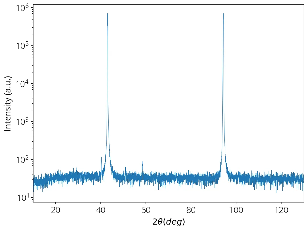
Plot
x = data[:, 0]
y = data[:, 6]

import matplotlib.pyplot as plt
%matplotlib inline

plt.semilogy(x, y, linewidth=0.5)
plt.xlabel("$2\\theta (deg)$")
plt.ylabel("Intensity (a.u.)")
plt.xlim(10, 130)
plt.show()
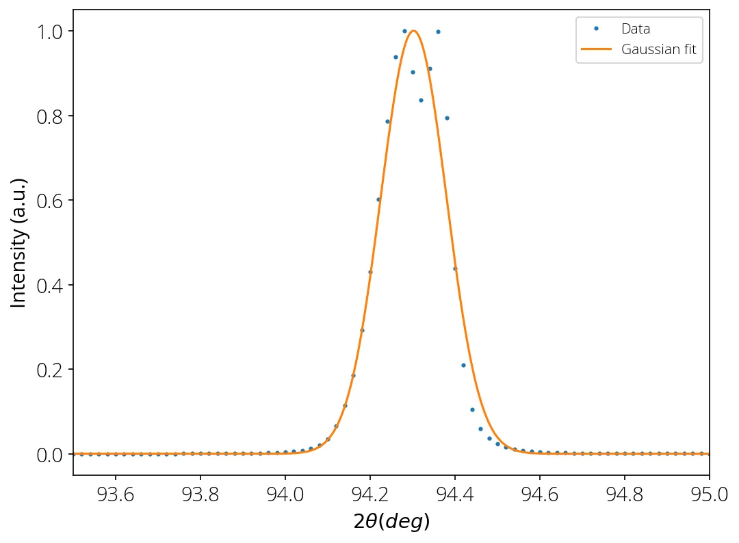
Fit Gaussian
x_fit, y_fit = suv.fit_gauss(x, y, xmin=93, xmax=95)
Output:
a = 725203.2202698857
x0 = 94.30231720686922
sigma = 0.07756533815550148
FWHM = 0.182666371356206
Let us plot the results:
plt.plot(x, y/max(y), 'o', markersize=2, label='Data')
plt.plot(x_fit, y_fit/max(y_fit), label='Gaussian fit')
plt.xlabel("$2\\theta (deg)$")
plt.ylabel("Intensity (a.u.)")
plt.xlim(93.5, 95)
plt.legend()
plt.show()
Locking peak position
Let us work with a XAS dataset. Here we want to lock the peak of second spectra at same energy as first spectra. We are interested only in the first peak, therefore limit the peak search to [525, 535]. If any limit is not provided, by default the program will search for maximum in the entire range.
s1 = suv.load("../dataset/sample_XAS.txt", 1)
s2 = suv.load("../dataset/sample_XAS.txt", 2)

s2 = suv.lock_peak(s2, s1, 525, 535)
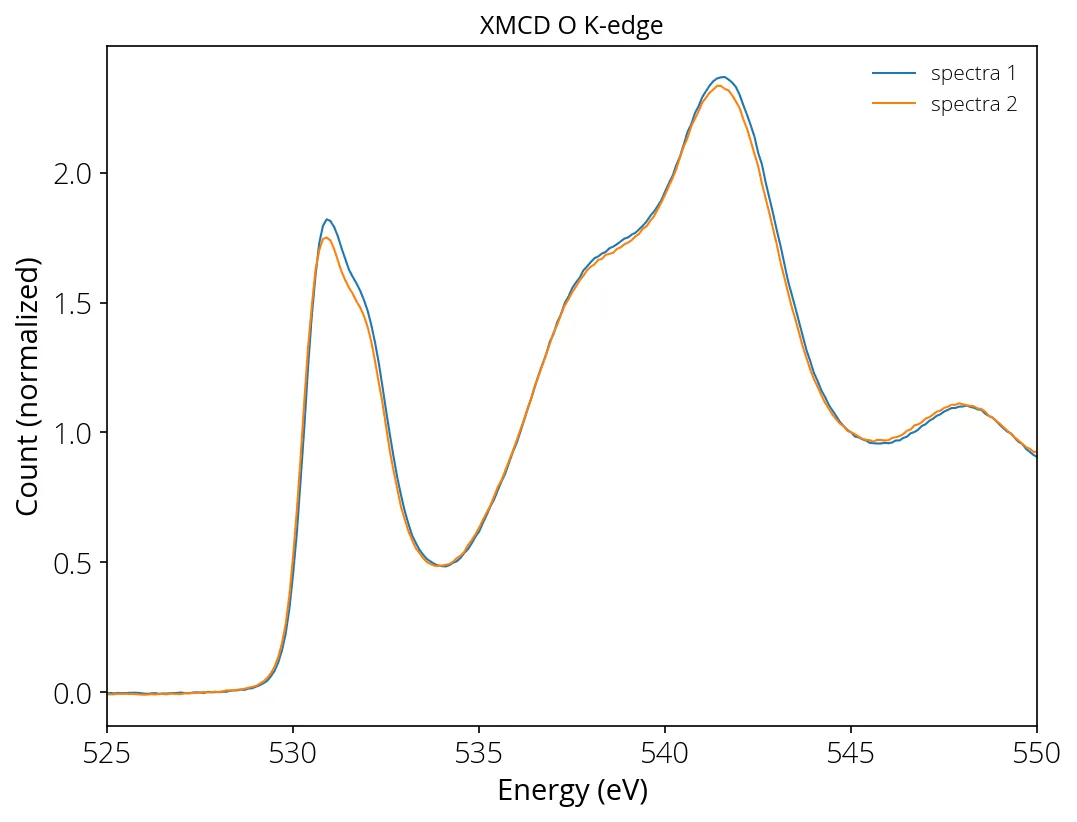
Background removal and normalization
The program removes linear background based on data values at energy point 520 eV and 528 eV (it finds two data point and calculates slope and intersection). Then normalize the intensity corresponding to energy value 545 eV (if the normalization location is not provided, the normalization is done at tail/end point).
i1 = suv.norm_bg(s1[:, 0], s1[:, 9]/s1[:, 4], 520, 528, 545)
i2 = suv.norm_bg(s2[:, 0], s2[:, 9]/s2[:, 4], 520, 528, 545)

# plot
plt.plot(s1[:, 0], i1, '-', linewidth=1, label="spectra 1")
plt.plot(s2[:, 0], i2, '-', linewidth=1, label="spectra 2")

plt.xlabel("Energy (eV)")
plt.ylabel("Count (normalized)")
plt.title("XMCD O K-edge")
plt.xlim(525, 550)
plt.legend(frameon=False)
plt.show()
If you want to normalize at the highest peak, you can find the energy value corresponding to the maximum intensity by:
energy_imax = s1[:, 0][np.argmax(s1[:, 9]/s1[:, 4])
Save plaintext
Say you want to save the energy and normalized intensity in plaintext to work in another plotting software.
import numpy as np

data = np.array([s1[:, 0], i1]).T
np.savetxt("data.txt", data)
Save CSV
We can save the full scan in a .csv file as well.
suv.save_csv("sample_data.txt", "data.csv", 12)
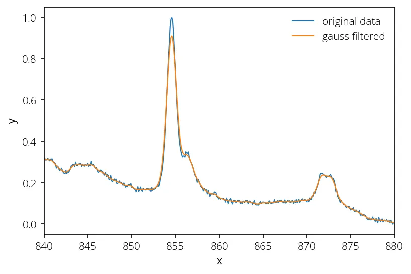
Curve smoothing
If the data is noisy, we can apply filters to smoothen it. Here is an example of applying Gaussian filter:
# import necessary packages
import numpy as np
import matplotlib.pyplot as plt
from scipy.ndimage.filters import gaussian_filter1d

%matplotlib inline
plt.rcParams["figure.dpi"]=150
plt.rcParams['figure.facecolor'] = 'white'

# load your data
data = np.loadtxt("data.txt")
x, y = data[:, 0], (data[:, 1] - min(data[:, 1]))/(max(data[:, 1]) - min(data[:, 1]))

# apply Gaussian filter to y
y_smth = gaussian_filter1d(y, sigma=2.5)

# make plots
plt.plot(x, y, lw=1, label="original data")
plt.plot(x, y_smth, lw=1, label="gauss filtered")
plt.legend(frameon=False)
plt.xlabel("x")
plt.ylabel("y")
plt.xlim(840, 880)
plt.show()