DFT+U calculation
We will calculate the density of states for NiO with and without including Hubbard . We will start from the example input file for NiO (check work directory under OpenMX installation).
src/NiO/NiO.in
#      File Name
#

System.CurrrentDirectory ./    # default=./
System.Name              nio
level.of.stdout          1    # default=1 (1-3)
level.of.fileout         1    # default=1 (1-3)
DATA.PATH                /home/svu/slspkd/openmx3.9/DFT_DATA19


# Definition of Atomic Species
#

Species.Number       2
<Definition.of.Atomic.Species
 Ni  Ni6.0S-s2p2d2f1     Ni_CA19S
 O   O5.0-s2p2d1         O_CA19
Definition.of.Atomic.Species>

<Hubbard.U.values                 #  eV
 Ni  1s 0.0 2s 0.0 1p 0.0 2p 0.0 1d 5.0 2d 0.0 1f 0.0
 O   1s 0.0 2s 0.0 1p 0.0 2p 0.0 1d 0.0
Hubbard.U.values>

<Hund.J.values                 #  eV
 Ni  1s 0.0 2s 0.0 1p 0.0 2p 0.0 1d 0.5 2d 0.0 1f 0.0
 O   1s 0.0 2s 0.0 1p 0.0 2p 0.0 1d 0.0
Hund.J.values>


# Atoms
#

Atoms.Number        4
Atoms.SpeciesAndCoordinates.Unit   AU # Ang|AU
<Atoms.SpeciesAndCoordinates
 1  Ni   0.0       0.0       0.0        9.5  6.5 off
 2  Ni   3.94955   3.94955   0.0        6.5  9.5 off
 3   O   3.94955   0.0       0.0        3.0  3.0 off
 4   O   3.94955   3.94955   3.94955    3.0  3.0 off
Atoms.SpeciesAndCoordinates>
Atoms.UnitVectors.Unit            AU  #  Ang|AU
<Atoms.UnitVectors
 7.89910   3.94955   3.94955
 3.94955   7.89910   3.94955
 3.94955   3.94955   7.89910
Atoms.UnitVectors>


# SCF or Electronic System
#

scf.XcType                 LSDA-CA     # LDA|LSDA-CA|GGA-PBE

# DFT+U part #
scf.Hubbard.U              On          # On|Off, default=off
scf.Hubbard.Occupation     dual        # onsite|full|dual, default=dual
scf.DFTU.Type		   2           # 1:Simplified(Dudarev)|2:General, default=1
scf.dc.Type                sFLL	       # sFLL|sAMF|cFLL|cAMF, default=sFLL
scf.Slater.Ratio           0.625       # default=0.625
scf.Yukawa		   off         # default=off
scf.SpinPolarization       On          # On|Off
scf.ElectronicTemperature  300.0       # default=300 (K)
scf.energycutoff           150.0       # default=150 (Ry)
scf.maxIter                200         # default=40
scf.EigenvalueSolver       band        # Recursion|Cluster|Band
scf.Kgrid                 6 6 6        # means 4x4x4
scf.Mixing.Type           rmm-diis     # Simple|Rmm-Diis|Gr-Pulay
scf.Init.Mixing.Weight     0.20        # default=0.30
scf.Min.Mixing.Weight      0.01       # default=0.001
scf.Max.Mixing.Weight      0.30        # default=0.40
scf.Kerker.factor          1.00        # default=1.00
scf.Mixing.History          5          # default=5
scf.Mixing.StartPulay       6         # default=6
scf.criterion             1.0e-7       # default=1.0e-6 (Hartree)


# MD or Geometry Optimization
#

MD.Type                     nomd       # Nomd|Opt|DIIS|NVE|NVT_VS|NVT_NH
MD.maxIter                   1         # default=1
MD.TimeStep                 0.05       # default=0.5 (fs)
MD.Opt.criterion          1.0e-4       # default=1.0e-4 (Hartree/bohr)


# Band dispersion
#

Voronoi.Charge		     on

Band.dispersion              off        # on|off, default=off
# if <Band.KPath.UnitCell does not exist,
#     the reciprical lattice vector is employed.
Band.Nkpath                1
<Band.kpath
  25  0.0 0.0 0.5   0.0 0.5 0.5   Z K
Band.kpath>


# MO output
#

MO.fileout                  off        # on|off
num.HOMOs                    1         # default=1
num.LUMOs                    1         # default=1
MO.Nkpoint                   1         # default=1
<MO.kpoint
 0.0  0.0  0.0
MO.kpoint>


# DOS and LDOS
#

Dos.fileout                 on         # on|off , default=off
Dos.Erange              -10.0  10.0    # default = -20 20
Dos.Kgrid                 9 9 9     # default = Kgrid1 Kgrid2 Kgrid3


# output Hamiltonian and overlap
#

HS.fileout                   off     # on|off, default=off
note
If the initial spin configuration is unpolarized for LDA+U calculations, it is
required to provide the switch for enhancement of orbital polarization in the
LDA+U method in the last column of Atoms.SpeciesAndCoordinates, on means
that the enhancement is made, off means no enhancement.
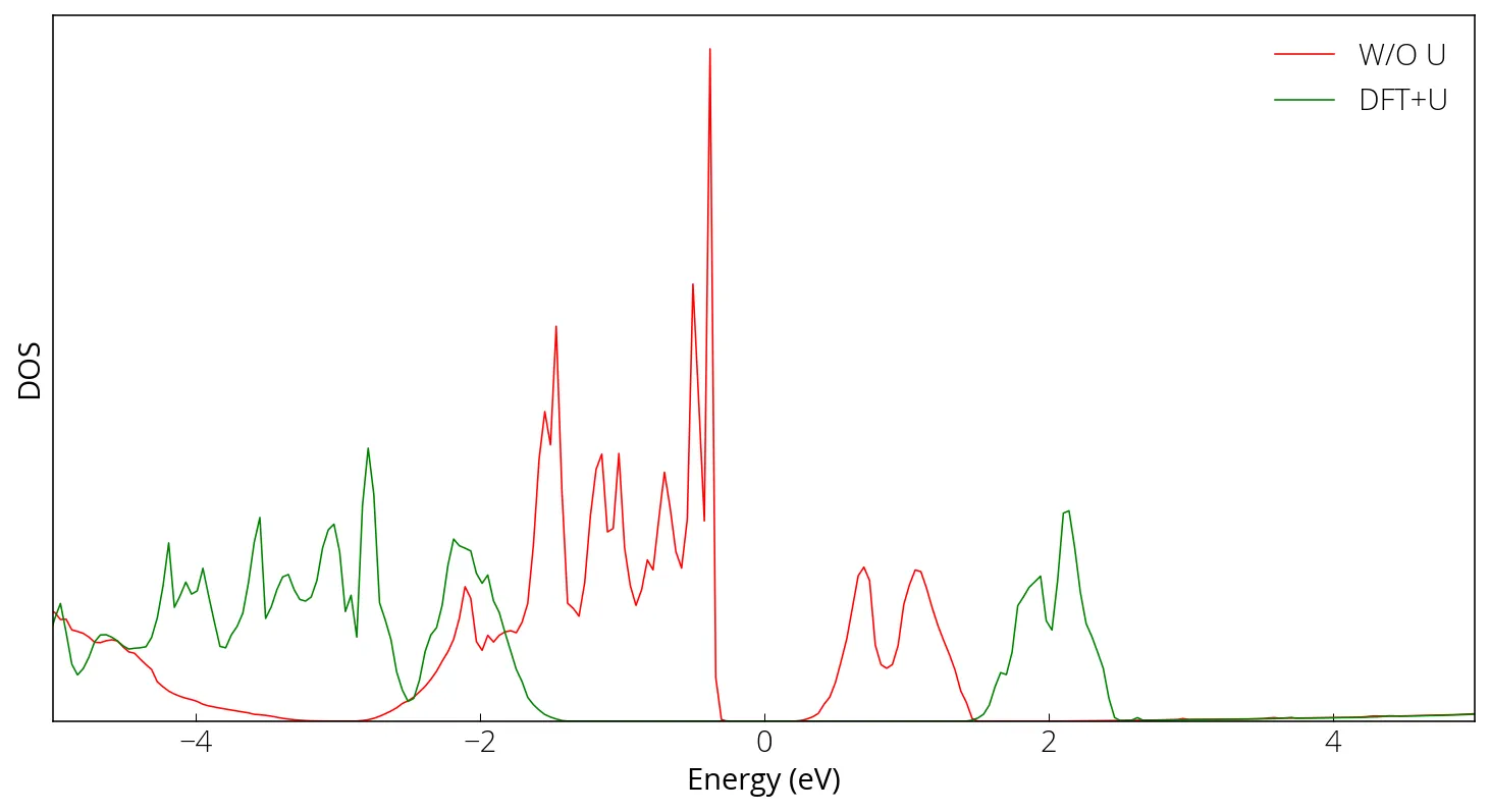
Here we compare the density of states with and without considering electronic correlation.
tip
If you have difficulty with SCF convergence, you might try
scf.Mixing.Type Rmm-Diish
which is suitable for the plus U method and the constraint schemes. Find more details here.