Spin-Orbit Coupling

In order to consider spin orbit coupling effect in our electronic structure calculation in quantum espresso, we need to use a full relativistic pseudo potential. Following settings are needed in the &SYSTEM card:

&SYSTEM
    ...
    noncolin = .true.
    lspinorb = .true.
    ...
/

Non collinear spin

In simple spin polarized calculation (nspin=2), the spin quantum number (up or down) is considered in the calculation. In non-collinear case, the spin has more degrees of freedom, and can be oriented in any direction. Non-collinear magnetism is quite common in nature, where the spins are not parallel (ferromagnetic) or anti-parallel (antiferromagnetic), rather they orient in spirals, helicoids, canted or disordered. Non-collinear magnetism can occur because of geometric frustration of magnetic interaction. It can also occur due to the magnetocrystalline anisotropy which is the result of interaction between the spin and lattice interaction. This relativistic effect comes via spin-orbit coupling.

We can constrain the magnetic moment:

&SYSTEM
  ...
  constrained_magnetization = 'atomic direction'
  ...
/

Starting magnetization can be specified by angle1 (angle with $z$ axis) and angle2 (angle of projection in $xy$-plane and with $x$-axis). Also check the penalty function ($\lambda$).

&SYSTEM
  ...
  angle1(i) = 0.0d0
  angle2(i) = 0.0d0
  lambda = 0.5
  ...
/

i is the index of the atom in ATOMIC_SPECIES card.

Strategy for convergence

Spin-orbit coupling calculations are often hard to converge. Use a smaller mixing_beta for such calculations. First perform a collinear calculation with non-relativistic pseudopotential, and then start from the obtained charge density to perform non-colinear spin orbit calculation.

&ELECTRONS
  ...
  mixing_beta = 1.0000000000d-01
  startingpot = 'file'
/

When starting with non-collinear calculation from an existing charge density file from a collinear lsda calculation, we need to set lforcet=.true.. It assumes previous density points in z direction, and rotates in the direction specified by angle1 (initial magnetization angle with $z$-axis in degrees), and angle2 (angle in degrees for projections in $xy$-plane and with $x$-axis).

&SYSTEM
...
  angle1(i) = 0.0
  angle2(i) = 0.0
  lforcet = .true.
/

Also, make sure that energy and charge density cutoffs are sufficient. Certain pseudo potentials might have issues, try with pseudo potentials from a different library. In case of metallic systems, remember to apply smearing.

Common Errors

• S matrix not positive definite: This error might appear due to numerical instability from overlapping atoms. Check atomic positions carefully. In one my calculations, this error was resolved after setting higher ecutrho.

• Simplified LDA+U not implemented with noncol magnetism, use lda_plus_u_kind=1.

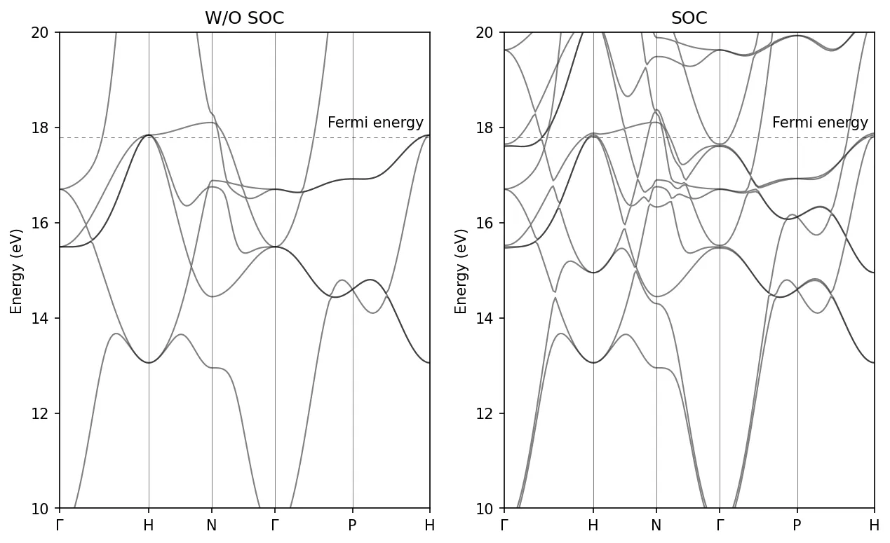
Bandstructure of Fe with SOC

src/fe/pw.scf.fe_soc.in

&control
   calculation='scf'
   pseudo_dir = '../pseudos/',
   outdir='./tmp/'
   prefix='fe'
/

&system
   ibrav = 3,
   celldm(1) = 5.39,
   nat= 1,
   ntyp= 1,
   noncolin=.true.,
   lspinorb=.true.,
   starting_magnetization(1)=0.3,
   ecutwfc = 70,
   ecutrho = 850.0,
   occupations='smearing',
   smearing='marzari-vanderbilt',
   degauss=0.02
/

&electrons
   diagonalization='david'
   conv_thr = 1.0e-8
   mixing_beta = 0.7
/

ATOMIC_SPECIES
Fe 55.845 Fe.rel-pbe-spn-rrkjus_psl.1.0.0.UPF

ATOMIC_POSITIONS alat
Fe 0.0 0.0 0.0

K_POINTS AUTOMATIC
14 14 14 1 1 1

Run the scf calculation:

mpirun -np 8 pw.x -i pw.scf.fe_soc.in > pw.scf.fe_soc.out

Prepare the input file for nscf bands calculation:

src/fe/pw.bands.fe_soc.in

&control
   calculation='bands'
   pseudo_dir = '../pseudos/',
   outdir='./tmp/'
   prefix='fe'
/

&system
   ibrav = 3,
   celldm(1) = 5.39,
   nat= 1,
   ntyp= 1,
   noncolin=.true.,
   lspinorb=.true.,
   starting_magnetization(1)=0.3,
   ecutwfc = 70,
   ecutrho = 850.0,
   occupations='smearing',
   smearing='marzari-vanderbilt',
   degauss=0.02
/
&electrons
   diagonalization='david'
   conv_thr = 1.0e-8
   mixing_beta = 0.7
/

ATOMIC_SPECIES
Fe 55.845 Fe.rel-pbe-spn-rrkjus_psl.1.0.0.UPF

ATOMIC_POSITIONS alat
Fe 0.0 0.0 0.0

K_POINTS tpiba_b
6
0.000  0.000  0.000  40  !gamma
0.000  1.000  0.000  40  !H
0.500  0.500  0.000  30  !N
0.000  0.000  0.000  30  !gamma
0.500  0.500  0.500  30  !P
0.000  1.000  0.000   1  !H

Run the bands calculation:

mpirun -np 8 pw.x -i pw.bands.fe_soc.in > pw.bands.fe_soc.out

Finally post process the bandstructure data:

src/fe/pp.bands.fe_soc.in

&BANDS
    outdir='./tmp/',
    prefix='fe',
    filband='fe_bands_soc.dat',
/

In this case spin_component has been removed and we add lsigma(3)=.true. that instructs the program to compute the expectation value for the z component of the spin operator for each eigenfunction and save all values in the file fe.noncolin.data.3. All values in this case are either +1/2 or -1/2.

mpirun -np 8 bands.x -i pp.bands.fe_soc.in > pp.bands.fe_soc.out

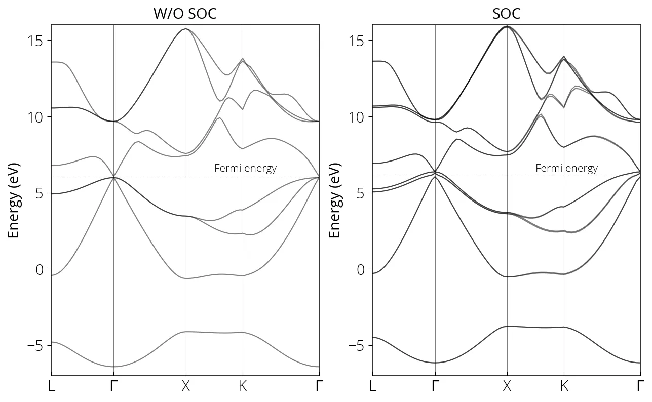
SOC calculation for GaAs

Please check the respective input files.

mpirun -np 8 pw.x -i pw.scf.GaAs_soc.in > pw.scf.GaAs_soc.out
mpirun -np 8 pw.x -i pw.bands.GaAs_soc.in > pw.bands.GaAs_soc.out
mpirun -np 8 bands.x -i pp.bands.GaAs_soc.in > pp.bands.GaAs_soc.out