Phonon dispersion
In Quantum Espresso, phonon dispersion is calculated using ph.x program, which
is implementation of density functional perturbation theory (DFPT).
Here are the steps for calculating phonon dispersion:
(1) perform SCF calculation using pw.x
&control
  calculation = 'scf'
  prefix = 'GaAs'
  pseudo_dir = '../pseudos/'
  outdir = './tmp/'
  verbosity = 'high'
  wf_collect = .true.
/

&system
  ibrav = 2
  celldm(1) = 10.861462
  nat = 2
  ntyp = 2
  ecutwfc = 80
  ecutrho = 640
/

&electrons
  mixing_mode = 'plain'
  mixing_beta = 0.7
  conv_thr = 1.0e-8
/

ATOMIC_SPECIES
  Ga 69.723    Ga.pbe-dn-kjpaw_psl.1.0.0.UPF
  As 74.921595 As.nc.z_15.oncvpsp3.dojo.v4-std.upf

ATOMIC_POSITIONS
  Ga 0.00 0.00 0.00
  As 0.25 0.25 0.25

K_POINTS {automatic}
  8 8 8 0 0 0
We perform the SCF calculation:
mpirun -np 4 pw.x -i pw.scf.GaAs.in > pw.scf.GaAs.out
-
Usually higher energy cutoff values are used for phonon calculation to get better accuracy.
-
In case of two dimensional systems, use
assume_isolated = '2D'in theSYSTEMnamelist to avoid negative or imaginary acoustic frequencies near point. Read more here.
(2) calculate the dynamical matrix on a uniform mesh of q-points using ph.x
&INPUTPH
  outdir = './tmp/'
  prefix = 'GaAs'
  tr2_ph = 1d-14
  ldisp = .true.
!  recover = .true.
  nq1 = 6
  nq2 = 6
  nq3 = 6
  fildyn = 'GaAs.dyn'
/
Run the calculation:
mpirun -np 4 ph.x -i ph.GaAs.in > ph.GaAs.out
The above calculation is computationally demanding. Our example calculation took about a whole day on a 2.6 GHz quad core processor.
You can restart an interrupted ph.x calculation with recover = .true. in the
INPUTPH namelist. You can cleanly exit an ongoing calculation by creating an
empty file with name {prefix}.EXIT.
(3) perform inverse Fourier transform of the dynamical matrix to obtain inverse
Fourier components in real space using q2r.x. Below is our input file:
&INPUT
  fildyn = 'GaAs.dyn'
  zasr = 'crystal'
  flfrc = 'GaAs.fc'
/
mpirun -np 4 q2r.x -i q2r.GaAs.in > q2r.GaAs.out
(4) Finally, perform Fourier transformation of the real space components to get
the dynamical matrix at any q by using matdyn.x.
&INPUT
  asr = 'crystal'
  flfrc = 'GaAs.fc'
  flfrq = 'GaAs.freq'
  flvec = 'GaAs.modes'
!  loto_2d = .true.
  q_in_band_form = .true.
  q_in_cryst_coord = .true.
/
5
0.500 0.500 0.500   20 ! L
0.000 0.000 0.000   20 ! G
0.500 0.000 0.500   20 ! X
0.375 0.375 0.750   20 ! K
0.000 0.000 0.000    1 ! G
mpirun -np 4 matdyn.x -i matdyn.GaAs.in > matdyn.GaAs.out
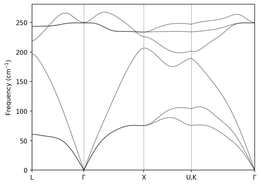
We can now plot the phonon dispersion of GaAs:
import numpy as np
import matplotlib.pyplot as plt

data = np.loadtxt("../src/GaAs-phonon/GaAs.freq.gp")

nbands = data.shape[1] - 1
for band in range(nbands):
    plt.plot(data[:, 0], data[:, band + 1], linewidth=1, alpha=0.5, color='k')
# High symmetry k-points (check matdyn.GaAs.in)
plt.axvline(x=data[0, 0], linewidth=0.5, color='k', alpha=0.5)
plt.axvline(x=data[20, 0], linewidth=0.5, color='k', alpha=0.5)
plt.axvline(x=data[40, 0], linewidth=0.5, color='k', alpha=0.5)
plt.axvline(x=data[60, 0], linewidth=0.5, color='k', alpha=0.5)
plt.xticks(ticks= [0, data[20, 0], data[40, 0], data[60, 0], data[-1, 0]], \
           labels=['L', '$\Gamma$', 'X', 'U,K', '$\Gamma$'])
plt.ylabel("Frequency (cm$^{-1}$)")
plt.xlim(data[0, 0], data[-1, 0])
plt.ylim(0, )
plt.show()
We may need to lower the value of conv_thr in scf calculation for more
accurate result.
Phonon Density of States
Input file for phonon DOS calculation:
&INPUT
  asr   = 'crystal'
  flfrc = 'GaAs.fc'
  flfrq = 'GaAs.dos.freq'
  flvec = 'GaAs.dos.modes'
  dos   = .true.
  fldos = 'GaAs.dos'
  nk1   = 25
  nk2   = 25
  nk3   = 25
/
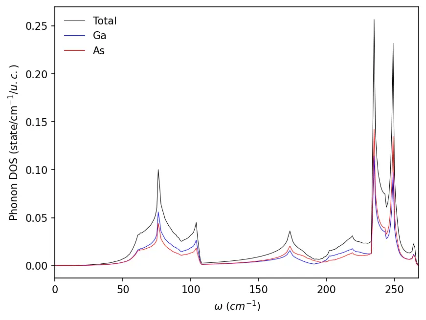
Plot phonon DOS:
freq, dos, pdos_Ga, pdos_As = np.loadtxt("../src/GaAs-phonon/GaAs.dos", unpack=True)

plt.plot(freq, dos, c='k', lw=0.5, label='Total')
plt.plot(freq, pdos_Ga, c='b', lw=0.5, label='Ga')
plt.plot(freq, pdos_As, c='r', lw=0.5, label='As')
plt.xlabel('$\\Omega~(cm^{-1}$)')
plt.ylabel('Phonon DOS (state/cm$^{-1}/u.c.$)')
plt.legend(frameon=False, loc='upper left')
plt.xlim(freq[0], freq[-1])
plt.show()