k-resolved DOS
Here we will calculate k-resolved density of states for silicon. First we begin with self consistent field calculation. Here is the input:
pw.x -inp si_scf.in > si_scf.out
Followed by the bands calculation. Note that for bands calculation I have doubled the number of k-points compared to our previous bands calculation.
pw.x -inp si_bands.in > si_bands.out
Calculate the orbital projections with k-resolved information:
src/silicon/si_projwfc.in
&projwfc
    outdir       = './tmp/'
    prefix       = 'silicon'
    ngauss       = 0
    degauss      = 0.036748
    DeltaE       = 0.005
    kresolveddos = .true.
    filpdos      = 'silicon.k'
/
projwfc.x -inp si_projwfc.in > si_projwfc.out
This will give separate orbital projections, as well as total sum for k-resolved DOS. Make plots:
notebooks/silicon-kpdos.ipynb
import matplotlib.pyplot as plt
from matplotlib import rcParamsDefault
import numpy as np
import zipfile
%matplotlib inline
# data file was compressed to reduce file size
zipobj = zipfile.ZipFile('../src/silicon/silicon.k.pdos_tot.zip', 'r')
zipdata = zipobj.open('silicon.k.pdos_tot')
data = np.loadtxt(zipdata)
k = np.unique(data[:, 0]) # k values
e = np.unique(data[:, 1]) # dos energy values
dos = np.zeros([len(k), len(e)])
for i in range(len(data)):
e_index = int(i % len(e))
k_index = int(data[i][0] - 1)
dos[k_index, e_index] = data[i][2]
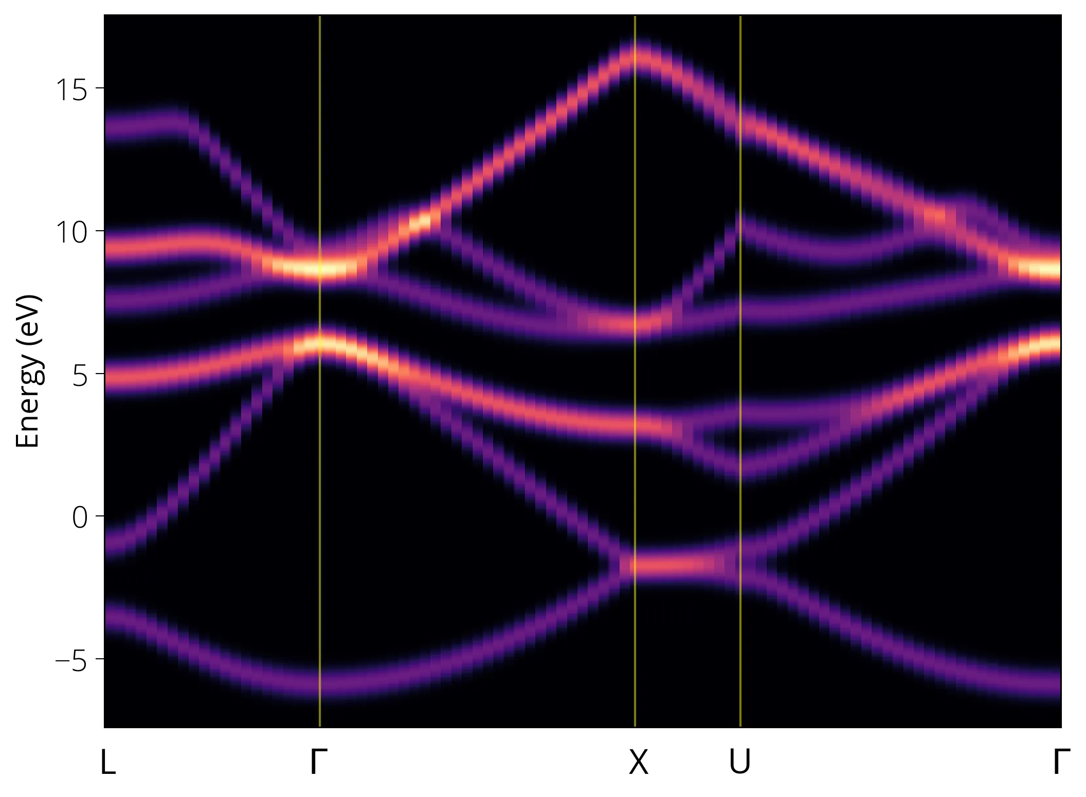
plt.pcolormesh(k, e, dos.T, cmap='magma', shading='auto')
# plt.ylim(-2, 10)
plt.xticks([])
plt.ylabel('Energy (eV)')
plt.xticks([])
plt.gcf().text(0.12, 0.06, 'L', fontsize=16, fontweight='normal')
plt.gcf().text(0.29, 0.06, '$\Gamma$', fontsize=16, fontweight='normal')
plt.gcf().text(0.55, 0.06, 'X', fontsize=16, fontweight='normal')
plt.gcf().text(0.63, 0.06, 'U', fontsize=16, fontweight='normal')
plt.gcf().text(0.892, 0.06, '$\Gamma$', fontsize=16, fontweight='normal')
plt.axvline(21, c='yellow', lw=1, alpha=0.5)
plt.axvline(51, c='yellow', lw=1, alpha=0.5)
plt.axvline(61, c='yellow', lw=1, alpha=0.5)
plt.show()
info
If you are using ibrav=0, you can calculate projwfc with lsym=.false.
option.
If we have contribution from multiple orbitals, we can sum desired projections
using sumpdos.x program. For example:
sumpdos.x *\(Cl\)*\(p\) > Cl_2p_tot.dat
This way we can plot different orbital projections along with energy and k-resolution.