Dielectric constant
First we perform self consistent field calculation:
mpirun -np 4 pw.x -i pw.scf.silicon_epsilon.in > pw.scf.silicon_epsilon.out
&CONTROL
  calculation = 'scf',
  prefix = 'silicon',
  outdir = './tmp/'
  pseudo_dir = '../pseudos/'
  verbosity = 'high'
/

&SYSTEM
  ibrav = 2,
  celldm(1) = 10.26,
  nat = 2,
  ntyp = 1,
  ecutwfc = 40
  nbnd = 20
  nosym = .TRUE.
  noinv = .TRUE.
/

&ELECTRONS
  mixing_beta = 0.6
  conv_thr = 1.0d-10
/

ATOMIC_SPECIES
  Si 28.086 Si.pz-vbc.UPF

ATOMIC_POSITIONS (alat)
  Si 0.0 0.0 0.0
  Si 0.25 0.25 0.25

K_POINTS automatic
6 6 6 0 0 0
Especially, notice following changes:
  nbnd = 20
  nosym = .true.
  noinv = .true.
We turn off the automatic reduction of k-points that pw.x does by using
crystal symmetries (nosym = .true. and noinv = .true.). This is because
epsilon.x does not recognize crystal symmetries, therefore the entire list of
k-points in the grid is needed. Secondly, we calculate a larger number of bands
(20), since we are interested in interband transitions. Also, note that
epsilon.x doesn't support the reduction of the k-points grid into the
irreducible Brillouin zone, so the PW runs must be performed with a uniform
k-points grid and all k-points weights must be equal to each other, i.e. in the
k-points card the k-points coordinates must be given manually in crystal or
alat or bohr, but not with the automatic option. However, the automatic
k-points option seems to work with nosym = .true. and noinv = .true.. If
required, we can perform nscf calculation with finer k-grid.
Next step is to prepare the input file for epsilon.x:
&inputpp
  outdir = "./tmp/"
  prefix = "silicon"
  calculation = "eps"
/

&energy_grid
  smeartype = "gauss"
  intersmear = 0.15
  intrasmear = 0.0
  wmin =  0.0
  wmax = 30.0
  nw = 1000
/
The variables smeartype and intersmear define the numerical approximation
used to represent the Dirac delta functions in the expression for
given above. For metals, we also need to use intrasmear broadening parameter,
usually 0.1 - 0.2 eV. The variables wmin, wmax and nw define the energy
grid for the dielectric function. All the energy variables are in eV.
mpirun -np 4 epsilon.x -i epsilon.si.in > epsilon.si.out
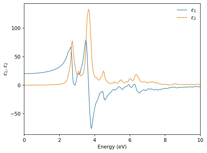
We will see the results are saved in separate .dat files. We can plot the real
() and imaginary () parts of dielectric constants:
import matplotlib.pyplot as plt
from matplotlib import rcParamsDefault
import numpy as np
%matplotlib inline
plt.rcParams["figure.dpi"]=150
plt.rcParams["figure.facecolor"]="white"

data_r = np.loadtxt('../src/silicon/epsr_silicon.dat')
data_i = np.loadtxt('../src/silicon/epsi_silicon.dat')
energy_r, epsilon_r = data_r[:, 0], data_r[:, 1]
energy_i, epsilon_i = data_i[:, 0], data_i[:, 1]

plt.plot(energy_r, epsilon_r, lw=1, label="$\\epsilon_1$")
plt.plot(energy_i, epsilon_i, lw=1, label="$\\epsilon_2$")
plt.xlim(0, 15)
plt.xlabel("Energy (eV)")
plt.ylabel("$\\epsilon_1~/~\\epsilon_2$")
plt.legend(frameon=False)
plt.show()
Ultra-soft pseudopotentials do not work with epsilon.x. Use norm-conserving
pseudopotentials. Also note that the above example is not tested against the
k-mesh. We usually need finer k-mesh for to converge. By default the
maximum number of k-points is set to 40000 in Quantum Espresso, if we need more
k-points, we can change Modules/parameters.f90 and recompile
Quantum Espresso.
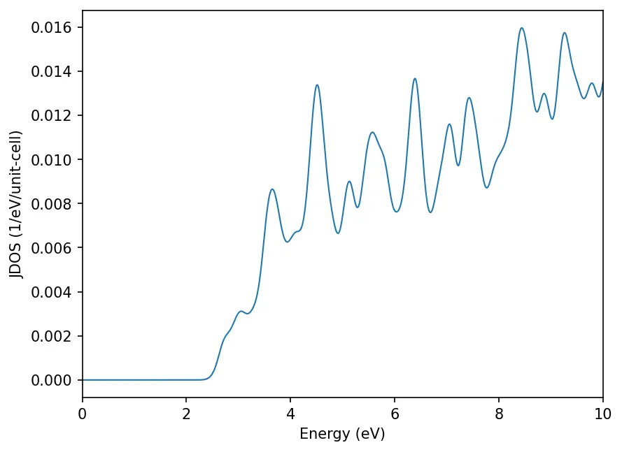
Joint Density of States
JDOS gives the number of states for a pair of initial and final states as a function of frequency (in eV). A larger intensity indicates a larger absorption in the absorption spectra. Input file for JDOS calculation:
&INPUTPP
  outdir      = "./tmp/"
  prefix      = "silicon"
  calculation = "jdos"
/

&ENERGY_GRID
  smeartype  = "gauss"
  intersmear = 0.15
  intrasmear = 0.0
  wmin       = 0.0
  wmax       = 10.0
  nw         = 1000
  shift      = 0.0
/
Sequence of steps to run:
mpirun -np 16 pw.x -in pw.scf.silicon_epsilon.in > pw.scf.silicon_epsilon.out
mpirun -np 16 pw.x -in pw.nscf.silicon_epsilon.in > pw.nscf.silicon_epsilon.out
mpirun -np 16 epsilon.x -in epsilon.jdos.si.in > epsilon.jdos.si.out