Density of States calculation

Electronic density of states is an important property of a material.

$\rho(E)dE$ = number of electronic states in the energy interval $(E, E + dE)$

Before we can run the Density of States (DOS) calculation, we need

Perform fixed-ion self consistent filed (scf) calculation. In plane-wave based DFT calculations the electronic density is expressed by functions of the form $\exp (i \textbf{k} \cdot \textbf{r})$ with energy given by $E = \hbar^2k^2/2m$ .
Perform non-self consistent field (nscf) calculation with denser k-point grid. A large number of $k$ points are required DOS calculation, as the accuracy of DOS depends on the integration in $k$ space.
Finally, the DOS can be determined by integrating the electron density in $k$ space.

I have created a new input file (pw.scf.silicon_dos.in) which is very much the same as our previous scf input file except some parameters are modified. You can find all the input files in my GitHub repository. We used the lattice constant value that we obtained from the relaxation calculation. We should not directly use the experimental/real lattice constant values. Depending on the method and pseudo-potential, it might result stress in the system. We have increased the ecutwfc to have better precision. We run the scf calculation:

pw.x < pw.scf.silicon_dos.in > pw.scf.silicon_dos.out

Next, we have prepared the input file for the nscf calculation. Where is have added occupations in the &system card as tetrahedra (appropriate for DOS calculation). We have increased the number of k-points to 12 × 12 × 12 with automatic option. Also specify nosym = .TRUE. to avoid generation of additional k-points in low symmetry cases. outdir and prefix must be the same as in the scf step, some of the inputs and output are read from previous step. Here we can specify a larger number of nbnd to calculate unoccupied bands. Number of occupied bands can be found in the scf output as number of Kohn-Sham states.

pw.x < pw.nscf.silicon_dos.in > pw.nscf.silicon_dos.out

Now our final step is to calculate the density of states. The DOS input file as follows:

src/silicon/pp.dos.silicon.in
&DOS
  prefix='silicon',
  outdir='./tmp/',
  fildos='si_dos.dat',
  emin=-9.0,
  emax=16.0
/

We run:

dos.x < pp.dos.silicon.in > pp.dos.silicon.out

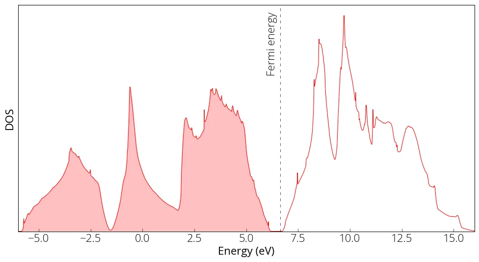
The DOS data in the si_dos.dat file that we specified in our input file. We can plot the DOS:

notebooks/silicon-dos.ipynb
import matplotlib.pyplot as plt
from matplotlib import rcParamsDefault
import numpy as np
%matplotlib inline

# load data
energy, dos, idos = np.loadtxt('../src/silicon/si_dos.dat', unpack=True)

# make plot
plt.figure(figsize = (12, 6))
plt.plot(energy, dos, linewidth=0.75, color='red')
plt.yticks([])
plt.xlabel('Energy (eV)')
plt.ylabel('DOS')
plt.axvline(x=6.642, linewidth=0.5, color='k', linestyle=(0, (8, 10)))
plt.xlim(-6, 16)
plt.ylim(0, )
plt.fill_between(energy, 0, dos, where=(energy < 6.642), facecolor='red', alpha=0.25)
plt.text(6, 1.7, 'Fermi energy', fontsize= med, rotation=90)
plt.show()

Important

For a set of calculation, we must keep the prefix same. For example, the nscf or bands calculation uses the wavefunction calculated by the scf calculation. When performing different calculations, for example you change a parameter and want to see the changes, you must use different output folder or unique prefix for different calculations so that the outputs do not get mixed.

tip

Sometimes it is important to sample the $\Gamma$ point for DOS calculation (e.g., the conducting bands cross the Fermi surface only at $\Gamma$ point). In such cases, we need to use odd k-grid (e.g., 9✕9✕5).