DFT+U calculation

Electronic structure for transition metals (with localized $d$ or $f$ electrons) is not accurately described by standard DFT, and therefore the need for DFT+U formulation.

&SYSTEM
    ...
    lda_plus_u = .TRUE.
    Hubbard_u(i) = 2.0
    ...
/

Here i refers to the atomic index in the &ATOMIC_SPECIES card corresponding to each ntyp. We can specify Hubbard_u(i) corresponding to more than one atom in separate lines.

There is also $U_{eff} = U - J$ implementation in QE. $J$ represents on-site exchange interaction. Number of $J$ terms depends on the manifold of localized electrons. For $p$, we have 1; for $d$, we have 2; and for $f$, we have 3 terms.

    ...
    lda_plus_u = .TRUE.
    lda_plus_u_kind = 1
    Hubbard_u(i) = U
    Hubbard_J(k, i) = J_{ki}
    ...

COMMON ERRORS

If you add Hubbard_u for elements that is not implemented to have $U$ term in QE, you might see a "pseudopotential not yet inserted" error.

Changes to input syntax in v7.1

Starting from Quantum Espresso version 7.1, there are changes to input syntax for DFT+U calculations. In the new version, instead of defining the necessary DFT+U parameters, now there is a new Hubbard card.

&system
...
-  lda_plus_u = .true.,
-  lda_plus_u_kind = 0,
-  U_projection_type = 'atomic',
-  Hubbard_U(1) = 4.6
-  Hubbard_U(2) = 4.6
...
/

+ HUBBARD (ortho-atomic)
+ U Fe1-3d 4.6
+ U Fe2-3d 4.6

Please refer to the qe-x.x/Doc/Hubbard_input.pdf for details.

DFT calculation for FeO

We will first perform the standard DFT calculation.

1. Perform the SCF calculation:

pw.x -in feo_scf.in > feo_scf.out

2. Perform NSCF calculation with denser k-grid:

pw.x -in feo_nscf.in > feo_nscf.out

3. Perform P-DOS calculation:

projwfc.x -in feo_projwfc.in > feo_projwfc.out

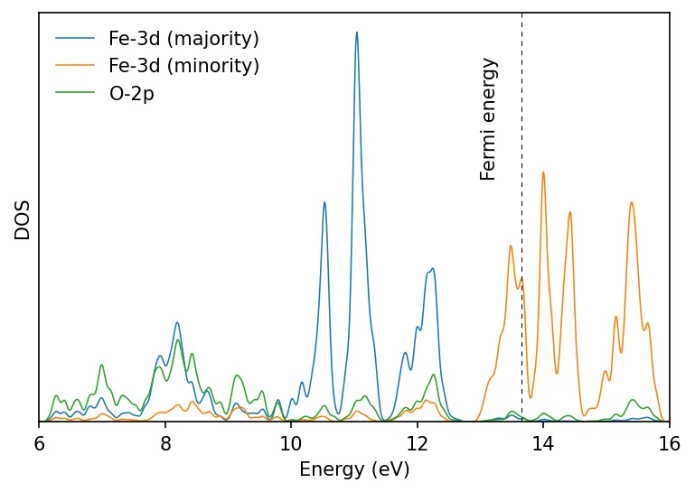
This gives us metallic density of states. In practice we get insulating FeO.

Calculating Hubbard U

src/FeO/feo_hp.in

&inputhp
   prefix = 'FeO'
   outdir = './tmp/'
   nq1 = 1, nq2 = 1, nq3 = 1
/

Perform a linear-response calculation using hp.x program:

hp.x -in feo_hp.in > feo_hp.out

Check the file FeO.Hubbard_parameters.dat.

info

1. We need to check the convergence against q-mesh (as well as k-mesh in SCF calculation). Here $1\times 1\times 1$ mesh is used. Important: lda_plus_u must be set to .true. during the SCF calculation, $U$ may be set to zero.

2. We can update the obtained $U$ value in our SCF calculation, and repeat linear response calculation until we have reached self consistency in $U$ value.

3. To go even further one can check the convergence of geometry during $U$ updates.

4. There is also inter-site Hubbard correction DFT+U+V calculation. The results could be more closer to hybrid functionals like GW. The $V$ can also be calculated using Quantum Espresso hp.x code.

5. Obtained value of $U$ depends on pseudopotential, Hubbard manifold (whether atomic, ortho-atomic etc.).

danger

The above hp.x code is not suitable for closed cell systems (e.g., fully occupied d-shell element), in such cases this linear response method gives unrealistically large $U$ value.

DFT+U calculation

We repeat the calculation after setting in the &SYSTEM card:

Hubbard_U(1) = 4.6
Hubbard_U(2) = 4.6

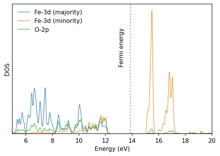
We repeat the above calculation and plot the results. Now we find insulating ground state.

info

U_projection_type = 'ortho-atomic' might give more realistic result than the default 'atomic'.

When performing $DFT+U$ calculation, the ground state might get stuck in a local minimum, in such cases we need to provide starting_ns_eigenvalue to help calculation reach desired/actual ground state. Please see these slides by Dr. Iurii Timrov for a relevant example.

tip

Here we have plotted the lpdos (local density of states). If we want to know the contribution of $d_{z^2}, d_{yz}, d_{x^2-z^2}$ ect., we can find them from the pdos columns. Also there arise important Lowdin charges information in the feo_projwfc.out file.

Resources

• Hands-on DFT+U by Iurii Timrov and Matteo Cococcioni
• Hubbard parameter calculation