Bandstructure Calculation

Before we can run bands calculation, we need to perform single-point self consistent field calculation. We have our input scf file with some new parameters:

src/silicon/pw.scf.silicon_bands.in
&CONTROL
  calculation = 'scf',
  restart_mode = 'from_scratch',
  prefix = 'silicon',
  outdir = './tmp/'
  pseudo_dir = '../pseudos/'
  verbosity = 'high'
/

&SYSTEM
  ibrav =  2,
  celldm(1) = 10.2076,
  nat =  2,
  ntyp = 1,
  ecutwfc = 50,
  ecutrho = 400,
  nbnd = 8,
!  occupations = 'smearing',
!  smearing = 'gaussian',
!  degauss = 0.005
/

&ELECTRONS
  conv_thr = 1e-8,
  mixing_beta = 0.6
/

ATOMIC_SPECIES
  Si 28.086 Si.pz-vbc.UPF

ATOMIC_POSITIONS (alat)
  Si 0.0 0.0 0.0
  Si 0.25 0.25 0.25

K_POINTS (automatic)
  8 8 8 0 0 0

Run the scf calculation:

pw.x < pw.scf.silicon_bands.in > pw.scf.silicon_bands.out

Next step is our band calculation (non-self consistent field) calculation. The bands calculation is non self-consistent and reads/uses the ground state electron density, Hartree, exchange and correlation potentials obtained in the previous step (scf calculation). In case of non self-consistent calculation, the pw.x program determines the Kohn-Sham eigenfunction and eigenvalues without updating Kohn-Sham Hamiltonian at every iteration. We need to specify the k-points for which we want to calculate the eigenvalues. You may use the See-K-path tool by materials cloud to visualize the K-path. We can specify nbnd, by default it calculates half the number of valence electrons, i.e., only the occupied ground state bands. Usually we are interested also in the unoccupied bands above the Fermi energy. Number of occupied bands can be found in the scf output as number of Kohn-Sham states. Below is a sample input file for the band calculation:

src/silicon/pw.bands.silicon.in
&control
  calculation = 'bands',
  restart_mode = 'from_scratch',
  prefix = 'silicon',
  outdir = './tmp/'
  pseudo_dir = '../pseudos/'
  verbosity = 'high'
/

&system
  ibrav =  2,
  celldm(1) = 10.2076,
  nat =  2,
  ntyp = 1,
  ecutwfc = 50,
  ecutrho = 400,
  nbnd = 8
 /

&electrons
  conv_thr = 1e-8,
  mixing_beta = 0.6
 /

ATOMIC_SPECIES
  Si 28.086  Si.pz-vbc.UPF

ATOMIC_POSITIONS (alat)
  Si 0.00 0.00 0.00
  Si 0.25 0.25 0.25

K_POINTS {crystal_b}
5
  0.0000 0.5000 0.0000 20  !L
  0.0000 0.0000 0.0000 30  !G
  -0.500 0.0000 -0.500 10  !X
  -0.375 0.2500 -0.375 30  !U
  0.0000 0.0000 0.0000 20  !G

Run pw.x with bands calculation input file:

pw.x < pw.bands.silicon.in > pw.bands.silicon.out

After the bands calculation is performed, we need some postprocessing using bands.x utility in order to obtain the data in more usable format. Input file for bands.x postprocessing:

src/silicon/pp.bands.silicon.in
&BANDS
  prefix = 'silicon'
  outdir = './tmp/'
  filband = 'si_bands.dat'
/

Run bands.x from post processing (PP) module:

bands.x < pp.bands.silicon.in > pp.bands.silicon.out

Finally, we run plotband.x to visualize bandstructure. We can either run it interactively (as described below) or provide an input file. In order to run interactively, type plotband.x in your terminal.

     Input file > si_bands.dat
Reading    8 bands at     91 k-points
Range:   -5.8300   16.3420eV  Emin, Emax > -6, 16
high-symmetry point:  0.5000 0.5000 0.5000   x coordinate   0.0000
high-symmetry point:  0.0000 0.0000 0.0000   x coordinate   0.8660
high-symmetry point:  1.0000 0.0000 0.0000   x coordinate   1.8660
high-symmetry point:  1.0000 0.2500 0.2500   x coordinate   2.2196
high-symmetry point:  0.0000 0.0000 0.0000   x coordinate   3.2802
output file (gnuplot/xmgr) > si_bands.gnuplot
bands in gnuplot/xmgr format written to file si_bands.gnuplot


output file (ps) > si_bands.ps
Efermi > 6.6416
deltaE, reference E (for tics) 4, 0
bands in PostScript format written to file si_bands.ps

You will have si_bands.ps with band diagram. Alternatively, you can use your favorite plotting program to make the plots. Below is an example of using Python matplotlib.

notebooks/si-bands.ipynb
import matplotlib.pyplot as plt
from matplotlib import rcParamsDefault
import numpy as np
%matplotlib inline

plt.rcParams["figure.dpi"]=150
plt.rcParams["figure.facecolor"]="white"
plt.rcParams["figure.figsize"]=(8, 6)

# load data
data = np.loadtxt('../src/silicon/si_bands.dat.gnu')

k = np.unique(data[:, 0])
bands = np.reshape(data[:, 1], (-1, len(k)))

for band in range(len(bands)):
    plt.plot(k, bands[band, :], linewidth=1, alpha=0.5, color='k')
plt.xlim(min(k), max(k))

# Fermi energy
plt.axhline(6.6416, linestyle=(0, (5, 5)), linewidth=0.75, color='k', alpha=0.5)
# High symmetry k-points (check bands_pp.out)
plt.axvline(0.8660, linewidth=0.75, color='k', alpha=0.5)
plt.axvline(1.8660, linewidth=0.75, color='k', alpha=0.5)
plt.axvline(2.2196, linewidth=0.75, color='k', alpha=0.5)
# text labels
plt.xticks(ticks= [0, 0.8660, 1.8660, 2.2196, 3.2802], \
           labels=['L', '$\Gamma$', 'X', 'U', '$\Gamma$'])
plt.ylabel("Energy (eV)")
plt.text(2.3, 5.6, 'Fermi energy', fontsize= small)
plt.show()

info

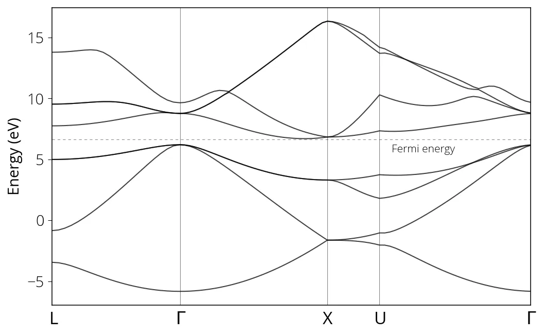
The k values corresponding to high symmetry points (such as $\Gamma$ , X, U, L) which we need to label in our band diagram, can be found in the post-processing output file (si_bands_pp.out).

Bandgap value can be determined from the highest occupied, lowest unoccupied level values printed in scf calculation output.

Note on bandgap

Usually, band gaps computed using common exchange-correction functionals such as LDA or GGA are severely underestimated compared to actual experimental values. This discrepancy is mainly due to (1) approximations used in the exchange correction functional and (2) a derivative discontinuity term, originating from the density functional being discontinuous with the total number of electrons in the system. The second contribution is larger contributor to the error. It can be partly addressed by a variety of techniques such as the GW approximation.

Strategies to improve band gap prediction at moderate to low computational cost now been developed by several groups, including Chan and Ceder (delta-sol)¹, Heyd et al. (hybrid functionals)², and Setyawan et al. (empirical fits)³.

Resources

M. Chan, G. Ceder, Efficient Band Gap Predictions for Solids, Physical Review Letters 19 (2010) https://doi.org/10.1103/PhysRevLett.105.196403 ↩
J. Heyd, J.E. Peralta, G.E. Scuseria, R.L. Martin, Energy band gaps and lattice parameters evaluated with the Heyd-Scuseria-Ernzerhof screened hybrid functional, Journal of Chemical Physics 123 (2005) https://doi.org/10.1063/1.2085170 ↩
W. Setyawan, R.M. Gaume, S. Lam, R. Feigelson, S. Curtarolo, High-throughput combinatorial database of electronic band structures for inorganic scintillator materials., ACS Combinatorial Science. (2011) https://doi.org/10.1021/co200012w. ↩

Note on bandgap​

Resources​

Footnotes​

Note on bandgap

Resources

Footnotes