DOS and bandstructure for Aluminum (metal)

Variable cell relaxation

First we are going to relax the cell and choose appropriate lattice constant for our chosen pseudo potential. In case of metals, it is important to provide smearing parameters in the input file.

src/al/al_vc_relax.in

&CONTROL
  calculation= 'vc-relax',
  prefix= 'al',
  outdir= '/tmp/'
  pseudo_dir = '../pseudos/'
  etot_conv_thr= 1e-6,
  forc_conv_thr= 1e-5
/

&SYSTEM
  ibrav=  2,
  celldm(1)= 7.652,
  nat=  1,
  ntyp= 1,
  ecutwfc = 50,
  ecutrho= 500,
  occupations= 'smearing',
  smearing= 'gaussian',
  degauss= 0.01
/

&ELECTRONS
  conv_thr= 1e-8
/

&IONS
/

&CELL
  cell_dofree= 'ibrav'
/

ATOMIC_SPECIES
  Al 26.981539 Al.pbe-n-rrkjus_psl.1.0.0.UPF

ATOMIC_POSITIONS (alat)
  Al 0.00 0.00 0.00

K_POINTS (automatic)
  10 10 10 0 0 0

We run pw.x to perform variable cell relaxation calculation:

pw.x < al_vc_relax.in > al_vc_relax.out

Now you may open the output file in vi editor and invoke search by pressing / and type Final enthalpy You will find the final lattice parameters below it.

Self consistent field (SCF) calculation

We obtain relaxed lattice constant = 7.652 * 0.498611683 / 0.5 = 7.63075 Bohr. We will use this value for our next step, self consistent calculation.

src/al/al_scf.in

&CONTROL
  calculation= 'scf',
  restart_mode= 'from_scratch',
  prefix= 'al',
  outdir= '/tmp/',
  pseudo_dir= '../pseudos/'
/

&SYSTEM
  ibrav= 2,
  celldm(1) = 7.63075,
  nat= 1,
  ntyp= 1,
  ecutwfc= 50,
  ecutrho= 500,
  occupations= 'smearing',
  smearing= 'gaussian',
  degauss= 0.01
/

&ELECTRONS
  conv_thr= 1e-8
/

ATOMIC_SPECIES
  Al 26.981539 Al.pbe-n-rrkjus_psl.1.0.0.UPF

ATOMIC_POSITIONS (alat)
  Al 0.00 0.00 0.00

K_POINTS (automatic)
  10 10 10 0 0 0

We run our self consistent calculation:

pw.x < al_scf.in > al_scf.out

Non-self consistent field calculation

Inspect the output file, and let's proceed to next step non-self consistent calculation:

src/al/al_nscf.in

&CONTROL
  calculation= 'nscf',
  restart_mode= 'from_scratch',
  prefix= 'al',
  outdir= '/tmp/',
  pseudo_dir= '../pseudos/'
/

&SYSTEM
  ibrav= 2,
  celldm(1) = 7.63075,
  nat= 1,
  ntyp= 1,
  ecutwfc= 50,
  ecutrho= 500,
  occupations= 'smearing',
  smearing= 'gaussian',
  degauss= 0.01
/

&ELECTRONS
  conv_thr= 1e-8
/

ATOMIC_SPECIES
  Al 26.981539 Al.pbe-n-rrkjus_psl.1.0.0.UPF

ATOMIC_POSITIONS (alat)
  Al 0.00 0.00 0.00

K_POINTS (automatic)
  40 40 40 0 0 0

Note the changes in input file. The calculation changed to nscf and we are now using a higher number of k-points grid.

pw.x < al_nscf.in > al_nscf.out

Density of states

Next we go ahead with our density of states calculation:

src/al/al_dos.in

&DOS
  prefix= 'al',
  outdir= '/tmp/',
  fildos= 'al_dos.dat',
  emin= -10,
  emax= 35
/

We run dos.x with DOS inputs:

dos.x < al_dos.in > al_dos.out

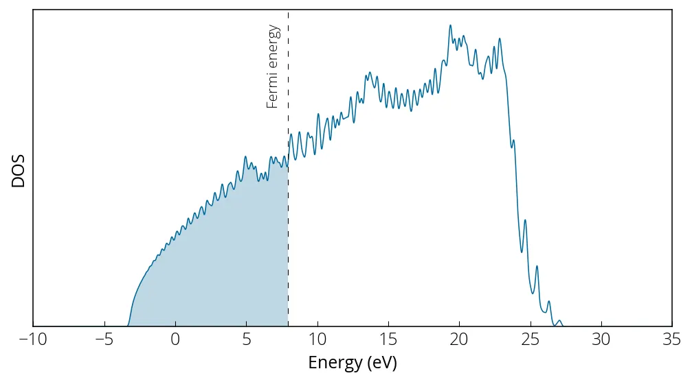
Note from our al_nscf.out that our Fermi energy is at 7.9421 eV. We plot our density of states:

Bandstructure calculation

We prepare the input file the same as the case of our previous example silicon:

src/al/al_bands.in

&CONTROL
  calculation= 'bands',
  restart_mode= 'from_scratch',
  prefix= 'al',
  outdir= '/tmp/',
  pseudo_dir= '../pseudos/'
/

&SYSTEM
  ibrav= 2,
  celldm(1) = 7.63075,
  nat= 1,
  ntyp= 1,
  ecutwfc= 50,
  ecutrho= 500,
  occupations= 'smearing',
  smearing= 'gaussian',
  degauss= 0.01
/

&ELECTRONS
  conv_thr= 1e-8
/

ATOMIC_SPECIES
  Al 26.981539 Al.pbe-n-rrkjus_psl.1.0.0.UPF

ATOMIC_POSITIONS (alat)
  Al 0.00 0.00 0.00

K_POINTS {crystal_b}
5
  00.000 0.500 00.000 20  !L
  00.000 0.000 00.000 30  !G
  -0.500 0.000 -0.500 10  !X
  -0.375 0.250 -0.375 30  !U
  00.000 0.000 00.000 20  !G

Followed by run pw.x:

pw.x < al_bands.in > al_bands.out

Now we proceed with post-processing:

src/al/al_bands_pp.in

&BANDS
  prefix = 'al'
  outdir = '/tmp/'
  filband = 'al_bands.dat'
/

And run bands.x:

bands.x < al_bands_pp.in > al_bands_pp.out

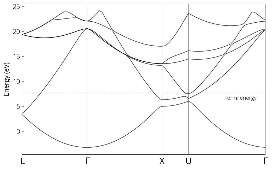
We obtain the following bandstructure:

Importance of smearing in convergence

Smearing is a technique used for suppressing unstable electron density in the calculation of metals. Such a problem occurs in metals (and semimetals) because the valence bands that cross Fermi level are partially occupied. Due to numerical accuracy, the electrons may occupy the unoccupied states during some iterations, making the algorithm unstable. In order to stablize the algorithm without using excessive number of k-points, smearing technique is used, which replaces the occupation number (either 0 or 1) is replaced by a smoothly varying function of energy. Such a smearing function could be Fermi Dirac distribution, instead of a step function (T = 0 K), we can use the finite temperature form.

Below we will test the convergence using PWTK against the number of k-points, three different smearing functions (Gauss, Methfessel-Paxton, and Marzari-Vanderbilt), and for various smearing values.

pwtk al.degauss.pwtk

We see that the m-v and m-p broadening allow for faster and smother convergence while depending less on degauss value than Gaussian broadening. The number suffix next to the legend labels are number of uniform k-points in Monkhorst-Plank grid.