Rotate Fermi map data

If your Fermi map measurement was not done keeping the high symmetry directions along the slit direction (or perpendicular to the slit direction), and you need to rotate the collected data in order to make the high symmetry directions along the x- or y-coordinate, the rotate_2d and rotate_3d functions come handy. Remember positive rotation angle rotates clockwise, and center of rotation is at ($k_x=0$, $k_y=0$).

rotate_2d can rotate a 2D array with respect to its surface normal. Let's get some Fermi map data first.

import arpespythontools as arp
import matplotlib.pyplot as plt
%matplotlib inline

url = 'https://pranabdas.github.io/drive/datasets/arpes/sample_map_data.zip'
data, energy, theta, phi = arp.load_ses_map(url)

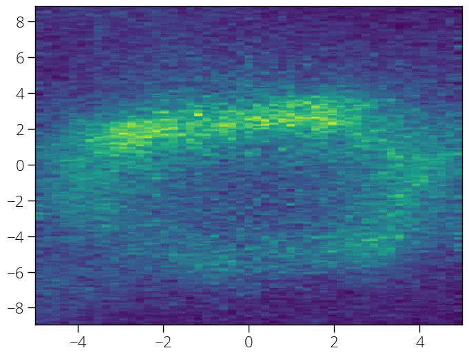
# Plot one slice
plt.figure(figsize = (8, 6))
plt.imshow(data[150, :, :], origin = 'lower', aspect = 'auto', \
    extent = (phi[0], phi[-1], theta[0], theta[-1]))
plt.show()

This is how a constant energy cut looks like before rotation:

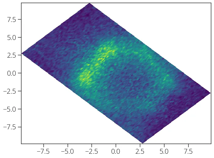
Now, we can rotate only a single slice first.

data_r, theta_r, phi_r = arp.rotate_2d(data[150, :, :], 45, theta, phi)

# Plot one slice
plt.figure(figsize = (8, 6))
plt.imshow(data_r, origin = 'lower', aspect = 'auto', \
    extent = (phi_r[0], phi_r[-1], theta_r[0], theta_r[-1]))
plt.show()

Let us plot a slice again. This is what we get after the rotation.

Rotate 3D Fermi map data

Instead of rotating only one slice, we can also rotate the full 3D array. rotate_3d function needs the 3D map data (with first dimension along the energy, second and third dimensions are $k_x$ and $k_y$, respectively) as input. It needs $k_x$ and $k_y$ vectors as input as well. Provide the required angle to rotate in degree as before. Axis of rotation is the first axis (i.e., energy). The function returns rotated data, new $k_x'$ and $k_y'$ vectors. Let's see an example:

data_r, theta_r, phi_r = arp.rotate_3d(data, 45, theta, phi)

# we can plot a slice after rotation to get the above result
plt.imshow(data_r[150, :, :], origin = 'lower', aspect = 'auto', \
    extent = (phi_r[0], phi_r[-1], theta_r[0], theta_r[-1]))
plt.show()