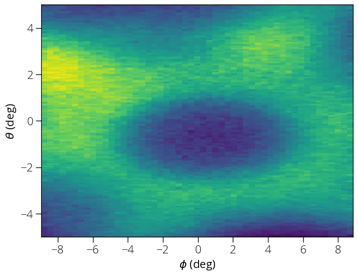
Slicing volume data

We can slice our 3D Fermi map data in order to get a particular plane using the plane_slice function. Say, we need a constant energy cut.

import arpespythontools as arp
data, energy, theta, phi = arp.load_ses_map('sample_map_data.zip')
# We want iso-energy surface integrated between energy values 15.6 and 15.8 eV
iso_energy_surf = arp.plane_slice(data, energy, 15.6, 15.8)

# Plot image
import matplotlib.pyplot as plt
%matplotlib inline
# Above line is specific to Jupyter Notebook
plt.figure(figsize = (8, 6))
plt.imshow(iso_energy_surf, origin = 'lower', aspect = 'auto', \
            extent = (theta[0], theta[-1], phi[0], phi[-1]))
plt.xlabel("$\\phi$ (deg)")
plt.ylabel("$\\theta$ (deg)")
plt.show()

This should give you an iso-energy surface like this:

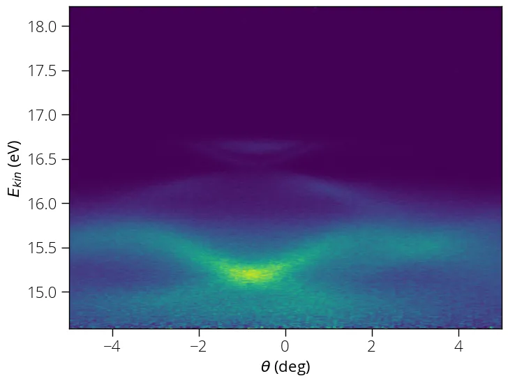
How about if we want the slice along another axis? All we need is transpose the data, and provide the correct axis order.

# integrating phi values between (-0.5, 0.5) degrees
phi_slice = arp.plane_slice(data.transpose([2, 0, 1]), phi, -0.5, 0.5)

# Plot image
import matplotlib.pyplot as plt
%matplotlib inline
# Above line is specific to Jupyter Notebook
plt.figure(figsize = (8, 6))
plt.imshow(phi_slice, origin = 'lower', aspect = 'auto', \
            extent = (phi[0], phi[-1], energy[0], energy[-1]))
plt.xlabel("$\\theta$ (deg)")
plt.ylabel("$E_{kin}$ (eV)")
plt.show()