Enhancing spectral features
Sometimes our spectra are not well resolved. In such cases, we may perform some post processing to enhance the spectral features.
Following modules are currently experimental and under development. Please review the codes and use with caution. You may instead use the Igor Macro implemented by Prof. P. Zhang.
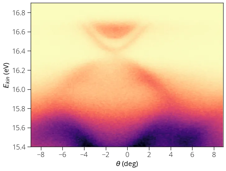
Here is how the original data looks like:
url = 'https://pranabdas.github.io/drive/datasets/arpes/sample_spectrum.txt'
data, energy, angle = arp.load_ses_spectra(url)

plt.imshow(data, origin = 'lower', aspect = 'auto', \
           extent = (angle[0], angle[-1], energy[0], energy[-1]))
plt.xlabel("$\\theta$ (deg)")
plt.ylabel("$E_{kin}$ (eV)")
plt.set_cmap('magma_r')
plt.show()
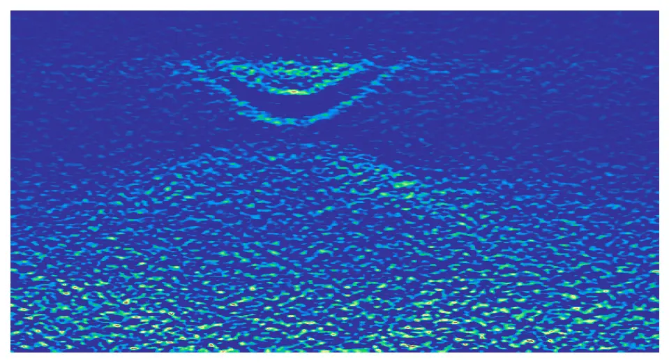
Laplacian
We can take the double derivative of the spectra in order to enhance the spectral features:
Since the and scales represent different quantities (units), we have a weight factor to account for this.
# diff2 = arp.laplacian(data, x, y, bw=5, w=1)
diff2 = arp.laplacian(data, energy, angle)

plt.imshow(diff2, vmax=0, cmap='terrain_r')
plt.axis('off')
plt.show()
2D curvature
The curvature method could be more appropriate to enhance spectral features. Two dimensional curvature is given by:
The details about the curvature method can be found here: P. Zhang et. al., A precise method for visualizing dispersive features in image plots, Review of Scientific Instruments 82, 043712 (2011).
# cv2d = arp.cv2d(data, x, y, bw=5, c1=0.001, c2=0.001, w=1)
cv2d = arp.cv2d(data, energy, angle)

plt.imshow(cv2d, vmax=0, cmap='terrain_r')
plt.axis('off')
plt.show()
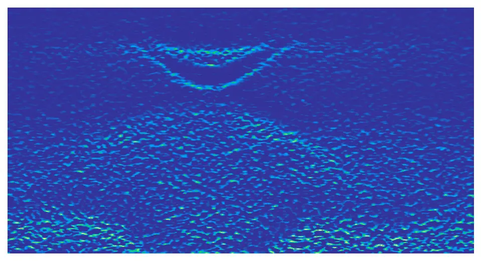
You may vary various free parameters (, , ) in order to get the best result specific to your dataset.